Mobile SLAM LiDAR vs. Terrestrial Laser Scanning (TLS): Accuracy vs. Speed on Job Sites
Author: Ruumica Engineering · Spatial Reality Capture & Systems
Published: October 31, 2026 · Category: Capture Technologies & Methodology
Selecting the wrong 3D laser scanning methodology for a commercial construction or industrial retrofit project leads to one of two expensive failures: deploying stationary tripod-mounted Terrestrial Laser Scanners (TLS) across compartmentalized multi-story buildings inflates field hours and surveying costs by 3x to 5x, whereas relying on unanchored mobile scanners for structural steel connections or long corridors introduces unacceptable trajectory drift. Modern reality capture engineering resolves this trade-off by matching sensor physics to project tolerances: Mobile SLAM LiDAR captures complex interiors at walking speed (2,000–5,000 m²/hour) with a relative local accuracy of ±2.0 mm to ±5.0 mm, while Terrestrial Laser Scanning (TLS) delivers ±1.0 mm to ±2.0 mm single-station precision and serves as a rigid geodetic control spine (L-EST97 / EH2000). This engineering benchmark equips chief engineers, BIM managers, quantity surveyors, and asset directors with objective decision criteria, 1,200 m² industrial field capture telemetry (35 minutes vs. 6 hours), SLAM loop-closure drift correction mathematics, and hybrid deployment protocols.
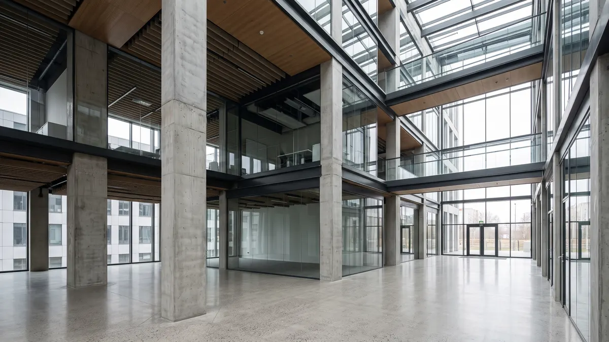
#Sensor Physics & Architecture: Static Tripod TLS vs. Dynamic 6-DoF SLAM Trajectories
Stationary Terrestrial Laser Scanning (TLS) measures 3D coordinates from fixed, leveled tripod setups using high-frequency Time-of-Flight (ToF) or phase-shift laser ranging at 1,000,000 to 2,000,000 points per second, achieving a single-station accuracy of ±1.0 mm to ±2.0 mm at ranges up to 130–350 meters. Mobile SLAM LiDAR (Simultaneous Localization and Mapping) computes a continuous 6-Degrees-of-Freedom (6-DoF) trajectory while the operator walks, fusing 320,000–640,000 points/sec multi-beam LiDAR with a 200–500 Hz Inertial Measurement Unit (IMU) and Visual-Inertial Odometry (VIO) to achieve ±2.0 mm to ±5.0 mm relative accuracy without a single tripod stop.
To evaluate how both instruments fit into a modern surveying pipeline (see our cornerstone Spatial Reality Capture Guide: LiDAR, Photogrammetry & 3DGS), we first establish their canonical technical definitions.
(x, y, z, roll, pitch, yaw) solved hundreds of times per second by LiDAR-Inertial-Visual Odometry (LIVO) to project raw laser range returns from the moving sensor frame into a unified global coordinate system."The Mechanics and Bottlenecks of Stationary TLS
A stationary terrestrial laser scanner (such as the Leica RTC360, Faro Focus Premium, or Trimble X9) rotates a precision mirror on a static tripod to record a dense spherical point cloud and HDR panoramic dome in 1.5 to 4.5 minutes per station. Because laser pulses travel strictly in straight lines of sight, every structural column, HVAC duct, partition wall, and equipment rack casts a geometric shadow (occlusion) behind it.
In a compartmentalized commercial asset — such as a hospital wing, school, historic Old Town building, or multi-level boiler house — the surveyor must physically pick up, move, and re-level the tripod every 4 to 10 meters while maintaining 35–50% cloud-to-cloud overlap through narrow doorways. Across a 60-room office floor, this translates into 80 to 120 tripod setups and a full day on site.
Tightly-Coupled LIVO Sensor Fusion in Mobile SLAM LiDAR
Survey-grade mobile SLAM instruments (such as the XGRIDS Lixel L2 Pro and NavVis VLX class systems operated by Allround) eliminate the tripod bottleneck through Tightly-Coupled LiDAR-Inertial-Visual Odometry (LIVO):
- Multi-Beam LiDAR Ranging: A rotating or non-repetitive multi-layer laser head continuously extracts planar and edge primitives (walls, floor slabs, structural beams) across a 360° field of view.
- Industrial-Grade IMU (200–500 Hz): High-frequency accelerometers and gyroscopes track micro-accelerations from the operator's gait, deskewing laser point returns in sub-millisecond intervals.
- Synchronized Visual Odometry & RTK-GNSS: Calibrated fisheye cameras track radiometric feature points to prevent longitudinal slip in geometrically repetitive corridors, while RTK-GNSS modules inject centimeter-level satellite fixes during outdoor facade transitions.
Engineering Specification Matrix: Mobile SLAM LiDAR vs. Stationary TLS vs. Hybrid Workflow
| Engineering Metric / Parameter | Mobile SLAM LiDAR (e.g., Lixel L2 Pro) | Stationary TLS (e.g., RTC360 / X9) | Allround Hybrid (TLS Spine + SLAM) |
|---|---|---|---|
| Relative / Single-Station Precision (1σ) | ±2.0 mm to ±5.0 mm (local room envelope) | ±1.0 mm to ±2.0 mm (within station range) | ±1.5 mm (structural nodes) / ±3.0 mm (rooms) |
| Global Accuracy per 100 m (Unanchored) | ±15.0 mm to ±35.0 mm (loop-dependent) | ±3.0 mm to ±8.0 mm (traverse-dependent) | ±2.0 mm to ±4.0 mm (rigidly locked) |
| Global Accuracy with GCP Network (L-EST97) | ±3.0 mm to ±8.0 mm | ±1.5 mm to ±3.0 mm | ±1.5 mm to ±3.5 mm |
| Laser Acquisition Rate (pts/sec) | 320,000 – 640,000 pts/sec | 1,000,000 – 2,000,000 pts/sec | Combined multi-resolution density |
| Real-World Field Capture Speed | 2,000 – 5,000 m² / hour | 180 – 450 m² / hour | 1,500 – 3,500 m² / hour |
| Surface Point Density (at 5 m range) | 15,000 – 60,000 pts/m² | 80,000 – 300,000+ pts/m² | 40,000 – 150,000 pts/m² (targeted zones) |
| Shadowing & Occlusion Risk | Minimal (continuous walk around obstacles) | High (requires extra stations behind pipes) | Virtually Zero (100% volumetric coverage) |
| 3D Gaussian Splatting (3DGS) Compatibility | Native (continuous video + LiDAR depth prior) | Limited (sparse static tripod panoramas) | Optimal (60 FPS 3DGS + millimeter BIM) |
#Field Benchmark Proof of Work: 1,200 m² Industrial & Office Facility (35 Minutes vs. 6 Hours)
In a controlled side-by-side field benchmark across a 1,200 m² industrial assembly and office facility in Tallinn, complete volumetric capture with Mobile SLAM LiDAR required 35 minutes of continuous walking (3 closed loops anchored to 8 Ground Control Points), whereas capturing the exact same asset with stationary Terrestrial Laser Scanning (TLS) required 68 tripod setups over 6 hours and 15 minutes. Cloud-to-cloud deviation analysis confirmed that the GCP-constrained SLAM point cloud achieved a Root Mean Square (RMS) deviation of 2.4 mm on structural walls and 3.1 mm on overhead roof trusses relative to the TLS baseline — well within the ±10 mm tolerance required for architectural LOD 300 Scan-to-BIM modeling.
To provide verifiable engineering telemetry (Proof of Work), Allround executed both capture pipelines across a mixed-typology facility comprising an 850 m² high-bay assembly hall (7.8 m clear height, overhead crane rails, steel roof trusses), a 200 m² two-story administrative wing (14 partitioned offices and stairwell), and a 150 m² dense district-heating and HVAC mechanical room.
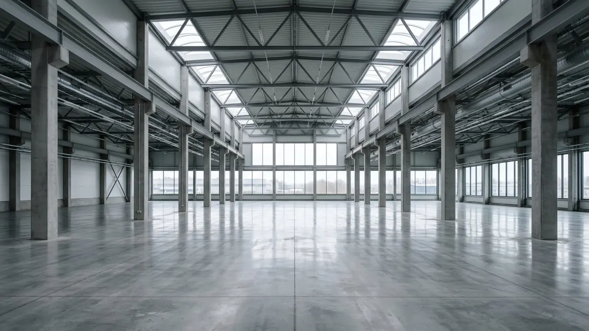
Figure 2: 1,200 m² industrial and office benchmark facility in Tallinn. Mobile SLAM LiDAR captured the entire complex (assembly bay, 14 office rooms, and MEP plant room) in 35 minutes at RMS ≤ 2.4 mm with zero operational downtime.
Side-by-Side Field Telemetry & Cost Breakdown (1,200 m² Benchmark Asset)
| Workflow Phase & Benchmark Metric | Method A: Mobile SLAM LiDAR (GCP-Anchored) | Method B: Stationary TLS (Tripod-Based) | Engineering Impact & Commercial Takeaway |
|---|---|---|---|
| 1. Geodetic Control Network (GCP) Deployment | 25 minutes (8 total-station targets in L-EST97) | 35 minutes (12 spheres & targets for traverse) | Both methodologies rely on a rigid geodetic control skeleton tied to national coordinates. |
| 2. Active On-Site Scanning Duration | 35 minutes (continuous walk at ~0.8 m/s, 3 loops) | 6 hours 15 minutes (68 tripod setups × ~5.5 min) | SLAM is 10.7x faster on site and eliminates production line shutdowns. |
| 3. Raw Dataset Volume & Office Registration (ICP) | 14.2 GB raw payload → 1.5 hours LIVO + GCP solve | 48.6 GB raw payload → 4.5 hours bundle registration | Compact raw data and continuous trajectory indexing save 3 hours of office compute. |
| 4. Volumetric Completeness in Dense MEP Zones | 99.4% (operator walked between boilers & ducts) | 91.2% (upper pipe crowns occluded from tripods) | Continuous mobile perspective eliminates blind spots behind dense mechanical piping. |
| 5. Verified Geometric Accuracy (RMS / 95% CI) | Local ±2.4 mm / Global ±4.2 mm | Local ±1.2 mm / Global ±2.1 mm | TLS is ~2 mm tighter on steel flanges; SLAM easily satisfies all LOD 200–300 BIM specs. |
| 6. Total Field Capture & Registration Cost | ~€780 + VAT (€0.65/m²) | ~€1,950 + VAT (€1.63/m²) | SLAM reduces baseline capture cost by 60%, preserving budget for BIM modeling. |
#SLAM Trajectory Drift Correction, Loop Closure, and Ground Control Points (GCP)
The primary engineering vulnerability of Mobile SLAM LiDAR is cumulative Inertial Measurement Unit (IMU) integration error — known as trajectory drift — which can accumulate to ±15 mm to ±35 mm along an unanchored 100-meter linear corridor. By enforcing closed-loop walking topologies (Loop Closure) and constraining the trajectory to total-station Ground Control Points (GCPs) spaced every 25 to 40 meters, non-linear Pose Graph Optimization locks the point cloud into national L-EST97 / EH2000 coordinates and compresses global drift down to ±3.0 mm to ±5.0 mm.
In long, featureless corridors, underground utility tunnels, or curtain-glazed office atriums (such as those in Ülemiste City and the Rotermann Quarter — see Indoor vs. Outdoor Capture Challenges: Overcoming Reflective Glass, Low Light, and Foliage), an uncalibrated one-way SLAM walk can cause corridor bowing or double-wall ghosting.
Allround prevents trajectory drift through a strict 4-Stage SLAM Metrology Protocol (detailed further in Point Cloud Density, Noise, and Registration: How Raw Scan Data is Cleaned and Aligned):
1. Figure-8 Closed-Loop Topologies: Our field engineers never terminate a scan pass in a dead-end room. Every floor plate is traversed in intersecting figure-8 loops that start and finish at the same benchmark, weaving multi-story stairwells into a continuous 3D lattice.
2. Total-Station GCP Anchors Every 25–40 Meters: Reflective survey targets are established along building perimeters, stair cores, and corridor intersections using a robotic total station. During the walk, the operator rests the SLAM reference base on each target plate for 3–5 seconds, injecting a hard coordinate constraint (X_L-EST97, Y_L-EST97, Z_EH2000) into the trajectory solver.
3. Global Pose-Graph Bundle Adjustment & Plane-to-Plane ICP: In post-processing, the optimization engine simultaneously minimizes LIVO odometry residuals, multi-pass planar ICP correspondences, and GCP anchor weights via min_T [ Σ ||e_LIVO(T_i, T_j)||²_Σ + Σ ||T_k · p_k − g_k^GCP||²_Λ ], where g_k^GCP is the surveyed benchmark coordinate and Λ_k enforces high-stiffness geodetic weighting.
4. Cross-Sectional Slice Verification Before Export: Prior to exporting .e57, .rcp, or .laz deliverables (see 3D File Formats Decoded: E57, LAS/LAZ, PLY, and SPZ Explained for Clients and Engineers), our engineers cut 10 mm orthogonal verification slices across the building's primary axes to verify that multi-pass structural walls resolve as a single razor-sharp profile.
#Engineering Decision Framework: When to Specify SLAM LiDAR, Stationary TLS, or a Hybrid Survey
Mobile SLAM LiDAR is the most cost-effective and technically appropriate choice for ~80% of architectural renovations, Scan-to-BIM modeling (LOD 200–300), and municipal building registry (EHR) permits where required dimensional tolerances range from ±5 mm to ±15 mm. Stationary TLS remains mandatory when contracts specify ±1.0–2.0 mm precision: prefabricated steel connection verification, ASTM E1155 concrete floor flatness audits, and long-range facade or bridge deformation monitoring. For complex commercial campuses and industrial plants, Allround's Hybrid TLS + SLAM + 3DGS protocol delivers the best of both worlds.
1. When Mobile SLAM LiDAR (with GCP Control) Wins
- Architectural Renovations & Scan-to-BIM (LOD 200–300): As-built modeling of commercial offices, residential apartments, schools, hospitals, and heritage buildings in Autodesk Revit or Graphisoft ArchiCAD (see our Scan-to-BIM & As-Built Modeling: The Complete Practical Handbook).
- Occupied Facilities & Zero-Downtime Environments: Active manufacturing plants, retail centers, hotels, and offices where scanning must be completed rapidly without disrupting operations.
- Estonian Building Registry (EHR) Permits & Area Audits: Retrospective building audits, occupancy permits (kasutusluba), fire-compartment verification, and BOMA/IPMS floor area certifications (see Reality Capture Project Planning: Scope, Budgeting, and Site Preparation).
- Real-Time 60 FPS 3DGS Digital Twins: Because mobile SLAM captures continuous multi-angle optical imagery synchronized with LiDAR depth, a single site walk produces both an engineering point cloud and an interactive 3D digital twin on the web hosted on
view.ruumica.com.
2. When Stationary Terrestrial Laser Scanning (TLS) Remains Mandatory
- Prefabricated Structural Steel & Glazing Fabrication (LOD 350–400): When off-site fabricated steel trusses, custom curtain-wall mullions, or modular MEP skids must bolt directly onto existing anchor plates with ±1.5–2.0 mm tolerance.
- Concrete Floor Flatness & Deflection Audits (FF/FL & ASTM E1155): Generating elevation contour heatmaps at 0.5 mm to 1.0 mm intervals for high-bay logistics slabs, where mobile SLAM sensor noise (±3 mm) would mask subtle slab waviness.
- Long-Range Sightlines (> 60–150 m) & Soaring Vaults (> 15–20 m): High industrial turbine halls, church vaults, bridges, dams, and multi-story exterior facades beyond the effective high-density range of handheld SLAM LiDAR.
- Multi-Epoch Deformation Monitoring: Periodic structural health monitoring requiring repeatable sub-2 mm station registration to detect foundation settlement or retaining wall tilt over time.
3. The Allround Hybrid Protocol (TLS Control Spine + Mobile SLAM Fill)
On large commercial and industrial assets (2,000 m² to 30,000+ m²), Allround combines both instruments in a unified Hybrid Reality Capture Architecture:
1. TLS Establishes the Rigid Geodetic Spine: We capture 8 to 15 high-precision stationary TLS setups along the building's primary structural corridors, central atrium, stair cores, and exterior perimeter to create a ±1.5 mm structural skeleton.
2. Mobile SLAM Captures the Compartmentalized Volume: Our engineers walk the secondary office bays, mechanical rooms, basements, and above-ceiling plenums using Mobile SLAM LiDAR.
3. Cloud-to-Cloud Trajectory Locking: During post-processing, the SLAM trajectory is rigidly constrained directly to the static TLS point cloud spine. This delivers TLS-grade global dimensional stability across the entire building while preserving SLAM's 10x capture speed, 100% occlusion-free coverage, and 50–65% lower field cost.
#Related Engineering Handbooks & Guides
This technical deep dive is part of Allround's Capture Technologies & Methodology library, anchored by our cornerstone Spatial Reality Capture Guide: LiDAR, Photogrammetry & 3DGS. Explore companion technical analyses and our foundational engineering handbooks below.
Specialized Deep Dives in Capture Technologies & Data Processing
| Specialized Technical Article | Engineering Focus & Practical Takeaways |
|---|---|
| What is 3D Gaussian Splatting (3DGS) and How Does It Compare to Photogrammetry Meshes? | Rasterizing continuous 3D ellipsoids at 60 FPS, Spherical Harmonics lighting, and capturing glass reflections and thin steelwork. |
| Point Cloud Density, Noise, and Registration: How Raw Scan Data is Cleaned and Aligned | Statistical outlier filtering (SOR), Iterative Closest Point (ICP) registration, and L-EST97 / EH2000 coordinate transformation. |
| Indoor vs. Outdoor Capture Challenges: Overcoming Reflective Glass, Low Light, and Foliage | Mitigating laser multipath reflections on glazing, dynamic exposure bracketing, and operating in Nordic winter conditions. |
| 3D File Formats Decoded: E57, LAS/LAZ, PLY, and SPZ Explained for Clients and Engineers | Compression benchmarks (8.4 GB E57 vs. 38 MB SPZ) and direct compatibility across Revit, ArchiCAD, AutoCAD, and WebGL viewers. |
Companion Ruumica Engineering Handbooks
| Handbook Title & Direct Link | Core Engineering Focus & Deliverables |
|---|---|
| Spatial Reality Capture Guide: LiDAR, Photogrammetry & 3DGS | Comparing Terrestrial Laser Scanning (TLS), Mobile SLAM LiDAR, and 3DGS radiance fields for AEC site verification. |
| Scan-to-BIM & As-Built Modeling: The Complete Practical Handbook | Translating registered laser point clouds into parametric Revit, ArchiCAD, and open IFC models at LOD 200–350. |
| Interactive 3D & Digital Twins on the Web: 3DGS and WebGL in Architecture | Streaming multi-million 3D Gaussian Splatting scenes in web browsers at 60 FPS via SOG/SPZ compression and Octree LoD. |
| Reality Capture Project Planning: Scope, Budgeting, and Site Preparation | Commercial scoping, €/m² pricing matrices, pre-scan job site readiness checklists, and EHR cadastral compliance. |
Ready to deploy the optimal balance of Mobile SLAM LiDAR speed, stationary TLS precision, and 60 FPS 3DGS visualization on your next commercial or industrial asset? Contact the Allround engineering team at info@ruumica.com or review our services and projects.